Want to do dynamics? This is how much it’ll cost.
I’m often asked what’s the biggest system we can simulate with Newton-X. You may guess, there is no definitive answer, as it depends on many variables, like the computational level and the simulation time.
We can, however, make a quick estimate on whether it’s feasible or not to do surface hopping dynamics for a particular system.
Technically, Newton-X doesn’t have any limitation concerning system size. The dynamic allocation of memory takes care of setting up all limits adequately. The main problem is computational cost.
The cost to run excited-state nonadiabatic dynamics with surface hopping depends on:
- how long it takes to compute energy plus energy gradients for a single geometry (let’s call it Tg in CPU-hours);
- how long the chemical process takes (Tp in fs);
- how much computational resources you have available.
Based on these quantities, you can do a simple estimate in this way:
To compute one single trajectory with time step Δt (also in fs), you need to compute Np = Tp/Δt single geometries.
Therefore, the computer time needed to simulate the trajectory is Tt = Np × Tg.
But you still need to compute Nt independent trajectories to have statistically relevant results. Then, the total computer time will be Ttotal = Nt × Tt.
Putting everything together,
Ttotal (CPU-hours) = Nt × Tp (CPU-hours) × Tg (fs) / Δt (fs).
For instance, suppose i) that it takes Tg = 1 CPU-hour to compute energy and gradients for a single geometry of your system, ii) that the chemical process you’re investigating takes place within 1 ps (Tp = 1000 fs), and iii) that you need Nt = 100 trajectories. Then, you may have to allocate:
Ttotal = 100 × 1 × 1000 / 0.5 = 200.000 CPU-hours.
I’ve few notes about this estimate:
First, I’m assuming that we have a quantum-chemical electronic-structure method able to get reasonable energies and energy gradients for any geometry visited during dynamics. This isn’t always true. If we use TDDFT, for instance, we won’t be able to describe conical intersections to the ground electronic state. You can know more about this in this paper.
Second, in the example, I took Nt = 100 trajectories. This is the typical number you find in the papers in this field. Note, however, that the maximum uncertainty associated to Nt is about ε = 1.96 × √(0.25/Nt) for a 95% confidence interval. For Nt = 100, this means ε = 0.098 ≅ 10%. If you are interested in a process that occurs with a frequency lower than 10%, you may need many more trajectories. (I discuss this issue in another post.)
Third, in the estimate, I also left out the time for computing the nonadiabatic couplings. This is a fair approximation for couplings based on wave-function overlaps and small double-ζ basis sets. However, a better estimate would be to take Tp = time(energy) + time(energy gradient) + time(couplings). Depending on the case, the computation of the couplings may take as much time as the computation of the energy gradients.
Well, our dynamics simulations will take 200.000 CPU-hours. This means 23 years in a single-core sequential run! Of course we need to consider parallelization. First, surface hopping is an independent-trajectory approach. It means that each trajectory may be run in different computers. We just put them together for analysis.
Thus, each trajectory in the example takes 2.000 CPU-hours, which means 3 months in single core or roughly 10 days in 8 cores. Therefore, if you have 800 cores available, you may have your simulations done within 10 days.
Finally, the current price of one CPU-hour in one of the French national high-performance clusters is about 0.044 €. This means that 200,000 CPU-hours will cost 8.800 €. Therefore, you must ask yourself: is it really worth doing dynamics?
MB
5 Comments
How many trajectories should I run? – Light and Molecules · April 18, 2018 at 1:42 PM
[…] do dynamics for such system and how many trajectories do I need. I addressed the first question in this post some time ago. Now, I want to quickly discuss the […]
Nuclear ensemble with importance sampling – Light and Molecules · May 4, 2018 at 3:47 PM
[…] of the computational cost is in the calculation of f, which is usually some electronic property like excitation energy or […]
Nonadiabatic Dynamics with Machine Learning – Light and Molecules · September 14, 2018 at 7:05 AM
[…] The rationale is that if the number of quantum-mechanical points needed to train the machine is significantly smaller than the total number of points spanned by dynamics, then ML could reduce the heavy computational cost of dynamics propagation. […]
Machine Learning Accelerates Excited-State Dynamics – Dr. Pavlo O. Dral · September 14, 2018 at 8:21 AM
[…] indispensable for better understanding and controlling them. Performing such simulations is however very costly. Additional complications arise from the necessity to take into account nonadiabatic […]
What is HPC and why do we need it? – EuroPAH · December 18, 2018 at 10:26 AM
[…] time on a French national supercomputer is about 0.044€ as reported in March 2017 here. The number is not huge, but if one consumes 1 million CPU hours then it becomes […]
Comments are closed.